Imagine a world where air is the coolest roller coaster you've ever seen. No rickety tracks, no screaming kids (except maybe you, as a scientist), just pure, unadulterated airflow. That's basically what we're about to build in SimScale, folks – a virtual wind tunnel for a pipe!
We're throwing a 12 m/s air tantrum at one end of this pipe (picture a toddler with a super soaker), and on the other side, it's wide open like a free buffet for hungry air molecules. Think of it as the ultimate escape room for air – no pressure, just freedom!
But here's the catch: this wild ride isn't just for kicks. We're using some fancy CFD (Computational Fluid Dynamics) mumbo jumbo to analyze exactly how this air behaves. We're talking twists, turns, pressure drops, the whole shebang. It's like having a microscopic army of air spies reporting back on every bump and jiggle in the journey.
So, grab your virtual goggles and get ready to blast off! We're about to see how a simple pipe can turn into a high-speed air adventure, all thanks to the magic of SimScale. Fasten your seatbelts, because science is about to get wild!
1) In the first step, we need to import our geometry that we will use in the analysis.It is best if it is a file type such as parasolid x_t, STEP or IGES.
2) In the next step, we create our simulation by pressing the CREATE SIMULATION key.
3) We have many types of CFD analyzes to choose from at SimScale. We want to make a simple simulation of gas flow in the pipe, for this purpose we select the INCOMPRESSIBLE type (red frame). If you want to learn about all other types of CFD analyzes available at SimScale, click HERE.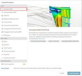
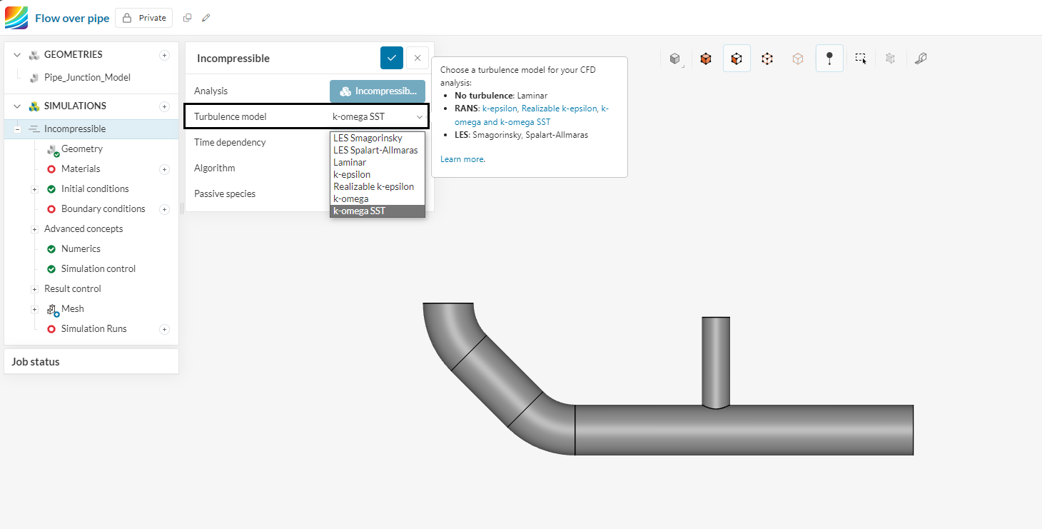
4) We then choose a turbulence model for the flow of our gas through the pipe. At SimScale we have several models to choose from. If you want to learn more about which model is suitable for your analysis - click HERE.
5) After selecting the turbulence model (k-omega SST by default) - we move on to defining the gas that will be in our pipe. For our simulation, we will assume ordinary STP air (standard temperature, pressure conditions).
6) Then we assign our model to the material, which will be air. If you want to learn more about material parameters in CFD SimScale, click HERE.
7) In the next step, you can define the initial simulation conditions for the gas domain. However, we will leave everything to the default settings. If you want to learn more about the types of initial conditions and why they are used, click HERE.
8) In this step, very important for every CFD analysis, we will establish the boundary conditions for our model. We will define two inlets, one as the initial gas velocity with a value of 12 m/s, the second as a free entrance to the Pressure Inlet model with an initial pressure value of 0 Pa and a free outlet also with a value of 0 Pa. If you want to learn more about the types of boundary conditions in CFD analysis in SimScale and when to use them, click HERE.
9) In the first step, we define Velocity Inlet with a value of 12 m/s according to the figure above. If you want to learn more about Velocity Type, click HERE.
10) We can further define the turbulence model in Velocity Inlet. However, we will leave this parameter in the default position. If you want to learn about the type of turbulence in this type of boundary condition (velocity inlet), click HERE.
11) Then we define a free Pressure Inlet with a value of 0 Pa. Why casual? Because the gas flow, in the direction of the pressure inlet or in the opposite direction, will depend on the remaining boundary conditions. We will be dealing with a suction phenomenon in the pressure inlet zone due to the higher pressure in the main pipe, which will suck gas from the pressure inlet to equalize the equilibrium state.
12) Then we define a pressure outlet, i.e. a free outlet (0 Pa) where the gas can go in both directions due to other defined boundary conditions. We can define pressure type here: mean value or fixed value. How do they differ? Click here. Done , we have defined entire model :) Now we go to the analysis settings.
13) In the next step, we go to the Numerics tab (red frame). There, we leave all parameters of the numerical analysis unchanged. If you want to learn more about what individual parameters are used for and when these parameters are used, click HERE.
14) In the next blunder we go to the Simulation Control option (black frame). Here we set the number of steps in our simulation, assign the number of processors, create calculation algorithms, etc. If you want to learn more about the individual options in Simulation Control, click HERE.
15) The next step is to set the meshing parameters. If you would like to learn more about how to control the quality of the mesh and how to model it for various types of simulations, click HERE. The figure below the presented parameters shows the default mesh generated for parameters that were not modified.
16) In Mesh Quality (red frame) you can check the quality of the generated mesh. You can precisely check the quality of finite elements on all sections of the model using the Iso-Volume function.
17) In the refinemets option, you can assume the density of model elements in the zones you are interested in. For CFD analyses, the density of elements is usually assumed on the walls where the greatest turbulence occurs, e.g. due to the phenomenon of friction. If you want to learn more about how to model the mesh, and more specifically about density in critical zones, click HERE.
18) After generating the mesh, you can check the mesh quality, number of nodes, number of elements and much more. If you want to learn more about individual items in the Event Log, click HERE.
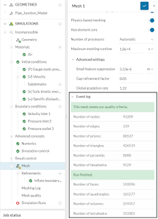
19) After generating a mesh with the refinement function, we can notice an increase in the number of finite elements at the walls of the model to be analyzed.
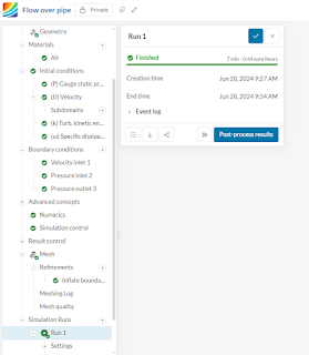
20) In the last step, we run the numerical analysis (red frame). We are shown the expected simulation time and the use of computing power. Click START.
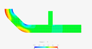
21) After performing the numerical analysis, click on Post-process results to see our results. In this post, we won't focus on generating results accurately. Below you can see example gas velocity distributions in the analyzed model.
22) Below are sample results for the longitudinal section of the model: velocity distribution, turbulent kinetic energy distribution.
Keywords for SimScale Pipe Airflow Analysis Tutorial:
General:
- SimScale, CFD (Computational Fluid Dynamics), Cloud-based simulation, Pipe airflow analysis, Tutorial, Geometry import (Parasolid, STEP, IGES), Simulation setup, Incompressible analysis, Turbulence model (k-omega SST), Fluid properties (air, STP),Material assignment, Initial conditions, Boundary conditions, Numerical settings, Simulation control, Meshing parameters, Mesh quality check (Iso-Volume), Mesh refinement, Mesh event log, Running the simulation, Post-processing results, Velocity distribution, Turbulent kinetic energy distribution, , Resources within SimScale, Basic airflow simulation


No comments:
Post a Comment