SimScale, as I mentioned in the previous post, is a revolutionary platform where, using only a browser, we are able to go through all stages of CFD modeling. We don't need costly working machines or any software investment. All it takes is a bit of willingness which, through the very friendly and intuitive SImScale interface, will lead us towards solving our problems related to fluid mechanics.
In today's post, which is divided into two parts, I would like to show you a single flow tutorial based on compressible gas. The configuration of two inlets and one outlet is to show you the interesting phenomenon of quasi-pump in inlet 2 caused by the main gas stream in inlet 1. More details below.
 |
| Compressible flow in SimScale |
The geometry for our analysis consists of two inlets and one outlet. For inlet 1, a gas outlet velocity of 30 m / s was defined. For inlet 2, an absolute pressure value of 1 atm was defined. The absolute pressure value of 1 atm was also defined for the model output. Pressure based boundary conditions are perfect options when there is gas movement in both directions on a boundary condition. The distribution of defined BC's is shown in the figure below.
 |
| BC's for CFD analysis |
First, you need to load the geometry for CFD analysis. It can be done, for example, in open source freeCAD program. Of course, if we have commercial solutions, they are also fully compatible with the SimScale software.
 |
| Import window for geometry file |
The second step is to choose the type of analysis depending on what phenomena we will deal with in our analysis.
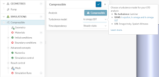
Our analysis is a single-phase flow of a compressible gas without the phenomena of heat transfer - so we choose the compressible flow. Thanks to the precise definition of our analysis, the program will select the optimal solvers so that the calculation time is as short as possible and the results are burdened with the lowest possible error.
The next step in CFD modeling is the selection of the type of analysis (steady, transient) and the turbulence model (viscosity). Due to the versatility and large turbulent flows in the model with two inlets, we choose the k-omega SST.
 |
| Type of solution and viscosity model (selection window) |
In the next step, we define the type of gas that will flow through our model. In the discussed case, it will be air with standard properties generally understood as STP (standard temperature pressure reference point).
 |
| Material type window definition |
Due to the fact that our simulation is greatly simplified and we model in steady mode, we do not define the initial conditions which we will leave on the default values of STP.
 |
| Initial conditions functions in SimScale |
A very important stage of modeling is to define the boundary and initial conditions. For our simple model, we will be dealing with three BC's. With two inlets and one outlet. The next three pictures below show the definition of these boundary conditions.
 |
| Inlet 2 parameters |
 |
| Inlet 1 parameters |
 |
| Outlet parameters |
In the next step, we define the accuracy of our analysis by setting the ceilings of partial equations and the margin of error for individual physical parameters (relaxation factors). The definition window of the above-mentioned parameters can be seen in the figure below.
 |
| Residuals and relaxation factors in SimScale |
In the next step, we define the number of iterations for our analysis and the size of a single step (time, iteration).
 |
| Definition of number of iterations and size of the time step (iteration for steady state) |
In the second part, I will present the meshing stage, launching the analysis and a simplified presentation of the results.
 |
| Compressible flow in SimScale |
A very important step in modeling, especially for steady state type of analysis, is discretization. SimScale offers a very transparent and intuitive panel for generating a mesh where using a slider we can define the number of finite elements (automatic) or using the size of a finite element (manual). We also have the ability to edit advanced discretization options which will be discussed in the next posts. After the discretization is done, we can see the quality of our mesh in the Meshing Log option.
 |
| Meshing window in SimScale |
 |
| Refining mesh in manual mode SimScale |
The last step before postporcessing is to initiate the computation. The simulation start window is presented below. SimScale offers an interesting option to save several analyzes for postporcessing into one simulation (multiple runs). I will also deal with this option in the next posts.
 |
| Run option in SimScale |
Of course, as in the commercial versions in SimScale, we can constantly observe the size of partial equations (and residuals) during the simulation. It is also possible to define your own monitors with the variables you are interested in.
 |
| Residual figure in SimScale |
As I mentioned at the beginning, thanks to the use of two inlets, the quasi-pump phenomenon is created in our model. This can be seen in the figure below where the gas in inlet 2 zone passes in both directions.
 |
| Vectors of gas flow in cross section area of model in SimScale |
The contours of the gas velocity distribution in the model on the cross-section are presented below.
 |
| Cross section velocity contour |
The figure below shows the velocity distribution along the X axis to clearly show the gas movement in two directions in the inlet 2 zone.
 |
| Velocity contours on X direction |
Temperature distribution on cross section of the model are presented below.
 |
| Temperature contour on cross section in SimScale |
All the details of the analysis performed can be traced in the Solver Log option (picture below).
 |
| Solver Log option in SimScale |


No comments:
Post a Comment